TABLE OF CONTENTS

2.3 Graphs of Exponential Functions

Goals:   The student will

• Graph by hand exponential functions (growth and decay) with different bases

• Be able to explain why exponential functions have a common vertical intercept

• Be able to discuss the properties of graphs of exponential functions, including domain, range, asymptote

• Understand the effect of changing the growth factor on the graph of an exponential function.

• Understand the effect of changing the initial value on the graph of an exponential function

Terms to know:  

·         Concave down

·         Concave up

·         Domain

·         Exponential function

·         Growth (or decay) factor

·         Growth (or decay) rate

·         Horizontal asymptote

·         Linear function

·         Range

·         Slope

Concept Prep:  Graphs of exponential functions

In this section we will look at the graphs of exponential functions.   Graphs of all exponential functions are similar in some ways, yet different in others.  The goal of this section is understand these similarities and differences.

In the concept prep assignment, your graph of  should look something like this:

The Effect of the Factor, a                       

I.   When the factor,  is greater than 1, we have an exponential growth function.   Your  

      graphs of  should look like this:

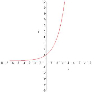
Note the following characteristics of graphs of functions of the form  where :

a)    They have a common y-intercept which is 1.  This means all these graphs go through the point (0,1).

                        Please understand WHY this is true.  Talk it over with your colleague. (HINT:  Substitute 0 in

                          for x in the formula.)

b)   Any real number can be the input.

                      We call the set of all possible inputs the domain of a function. The domain

                      of these exponential functions is, therefore,  .

c)    The output is never negative, nor is it 0.

                      We call the set of all outputs of a function the range. The range, then, of           

                      these exponential functions is .

                      Why is the output never negative?  Will this always be the case?

d)   Though the output is never negative or 0, as  gets bigger and bigger, but  is NEGATIVE (we write  ), the value of  gets very, very close to 0.  Take a look at this table of values for  to convince yourself:

x

2^x

x

2^x

0

1

-30

9.3132E-10

-1

0.5

-40

9.0949E-13

-2

0.25

-50

8.8818E-16

-3

0.125

-60

8.6736E-19

-4

0.0625

-70

8.4703E-22

-5

0.03125

-80

8.2718E-25

-10

0.000976563

-90

8.0779E-28

-20

9.5367E-07

-100

7.8886E-31

           Note that , a      

           mighty small number.   Symbolically, mathematicians would write:

           Since y approaches 0 as x gets large in the negative direction, we say the line     

            is a horizontal asymptote  for the graph of the function.

e)    The output values are increasing over the entire domain.  This means that as the x s

           get larger, as we move from left to right on the horizontal axis,  the ys also get

           larger. 

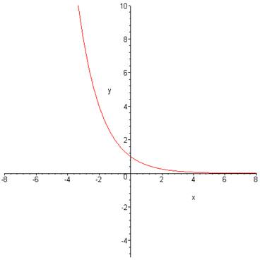
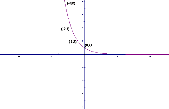
II.       When the factor, , is less than 1 but greater than 0, we have an exponential decay function.   Suppose that we have a scenario where after each time period, we have  of the previous value  left.  If the initial amount was 1, the following table shows the output values for various values of the input.

x

0

1

1

 1/2

2

 1/4

3

 1/8

4

   1/16

5

   1/32

x

-5

32

-4

16

-3

8

-2

4

-1

2

Plotting these values on a graph gives us the following.

Note that the characteristics of the graph of the function are similar to those mentioned for functions where : 

a)     It has a y-intercept which is 1.  This means that the graph goes through the point (0,1).

b)   Any real number can be the input.  This means that the domain is .

c)    The output is never negative, nor is it 0. This means the range is  .

d)   The line  is a horizontal asymptote of the graph.  This time, though, the outputs approach 0 as the inputs approach positive infinity:

                                                             .

       e)   The output values are decreasing over the entire domain.  This means that as the xs get larger, as we move from left to right on the horizontal axis,  the ys get smaller. 

      Checkpoint: Graphs of Exponential Functions 1

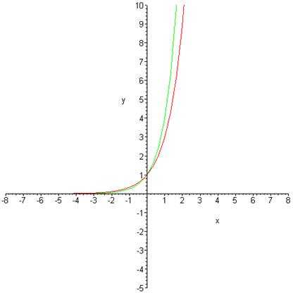
The Effect of the Initial Value, C

Class Activity:

Plot each of the following sets of graphs on one grid.  Comment on the effect of the initial value, C,  on the shape of the graph of .  Be sure to choose enough points so that you are certain that your graph is accurate.

1.                               2.                                3.    

The Effect of Adding a Constant, k

Class Activity:

Plot each of the following sets of graphs on one grid.  How does the constant affect the location of the horizontal asymptote?  Be sure to choose enough points so that you are certain that your graph is accurate.

1.                                  2.                    3.    

Exponential Graphs and Concavity

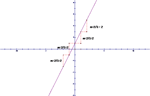
As we have noticed, the graphs of exponential functions curve upward.  These are very unlike the graphs of linear functions which are straight lines.

Recall also that the average rate of change of a linear function is constant.  We call this average rate of change slope.  Here’s a sketch to refresh your memory.

Note that for any two points we choose on the line, the slope (average rate of change) is the same.

A quite different situation occurs when we examine the graph of an exponential function.  Let’s again look at the graph of  and note the rates of change between points.

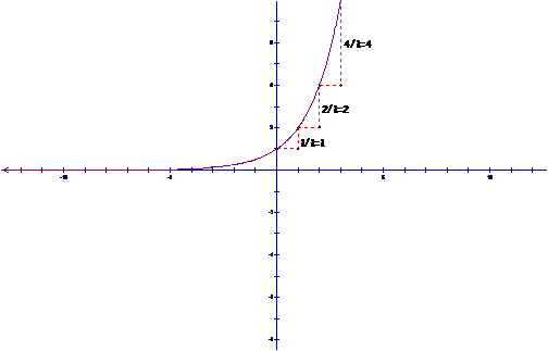
Notice that if we take the , we do NOT obtain the same value given different sets of points.  This graph is concave up.  A graph is concave up if the graph turns left (counterclockwise) as you travel along the curve from left to right.  Such graphs have the property that if you find the average rate of change over two intervals, with one interval lying (entirely) to the right of the other, the average rate of change over the interval to the right will be greater. For the sake of simplicity, we can begin with  and let the change in x equal 1.  

Below is the graph of .   Would you expect the average rate of change to be increasing, decreasing, or constant as the value of x increase? 

Find the average rate of change for the points listed in the graph and see if your conjecture was correct.

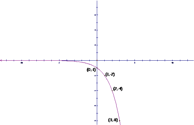
Just as a side note, not all graphs are concave up, even though the exponential graphs we looked at above are.    Graphs can turn to the right (clockwise) as you travel along the curve from left to right and we say such graphs are concave down.    The graph of  is one example.

Find the average rate of change between each of the points listed.  What do you notice about it as the value of x increases?

        Checkpoint: Graphs of Exponential Functions 2

More worked examples

Homework problems